Five Forecasts, One Market: How We See Around Corners

Markets are complex, and no single model can capture that complexity perfectly. A forecast based on historical patterns might miss a fundamental shift. A model built on cattle futures might overlook cut-specific demand. A structural model might miss what the market is already pricing in. Rather than expecting one approach to have all the answers, DecisionNext uses four weekly models and one daily model to understand the beef market, each asking different questions about the same market.

This approach takes more work to interpret, but it gives you something significantly more valuable than a single forecast: it shows you where the consensus is strong and where it’s uncertain. In this article, we explain how each model works and how to use them together to make confident decisions.

DecisionNext’s five beef forecasting models

Machine Learning (ML) (Weekly): Analyzes the cut’s own history, seasonality, and statistical relationships, best when cut-specific demand signals are strongest.

CME (Weekly): Uses live cattle futures to forecast the cut, relevant when cattle supply or futures expectations are driving the market.

Fundamentals (Weekly): Relates the cut to cattle using DecisionNext’s structural forecast (feed costs, herd dynamics, supply/demand), captures upstream drivers the futures may miss.

Cutout (Weekly): Anchors to boxed-beef cutout rather than cattle, provides a carcass and beef-demand perspective when boxed-beef and processing margins diverge from live cattle.

ML (Daily): Analyzes the cut’s own history at a daily frequency, with seasonality, and statistical relationships, best when near-term cut-specific demand signals are strongest. 

Why so many models?

Quite simply, a mathematical or statistical model is a collection of information measured through variables and data points. The only information the model “knows” is what is contained in those measurements. In the past, which information was used to feed those models was chosen by “modeling experts”, because there was no systematic way to have algorithms select the best set of information. Now with ML models, we can remove bias introduced by the modeler and let algorithms find relationships before the expert could. However, even with these cutting edge methods, models can use only a limited number of variables without weakening their explanatory or forecasting power. Too many variables can lead the model to attribute outcomes to factors that did not cause them. This is called overfitting and poses a major forecasting challenge.

Overfitting is also why many LLM forecasts can fail to accurately explain what is happening in markets. They have access to more information than any individual could consider, but without the right structure and reasoning, they can confidently explain and predict almost anything, even if the reasoning or logic is unsound. More information doesn’t improve their explanations or forecasts; with so much data, they can rationalize any outcome, correctly or not. In contrast, the DecisionNext ML forecast uses market-specific structure and statistical constraints to prevent this problem.

The key to preventing overfitting and building the most accurate forecast models is to ensure the modeling process uses the right reasoning and structure to reveal what can be learned about the markets.

How to use the five forecasts to understand the market: through the lens of the 90% lean beef market

We suggest starting with the weekly forecasts because this sets the foundation for understanding what has happened and what is likely to happen. While the daily forecasts are useful to understanding the day to day, the weekly forecast helps to reveal the broader trends as markets unfold. 

The DecisionNext weekly ML forecast, which does not rely on human judgement and bias, detects predictive relationships in variables before any human could. The model’s strengths and limitations are that it can only capture and use what has happened consistently over time. This means big one-time shocks or persistent trends can challenge forecast accuracy because it may assume the trend will continue indefinitely or miss major shifts that are expected but not explicitly measured in the data. To see what we mean by this, see the history of our ML forecasts (colorful squiggly lines that are updated each week) against the realized value (dark line) since July for domestic fresh 90% lean trim (Fig. 1).

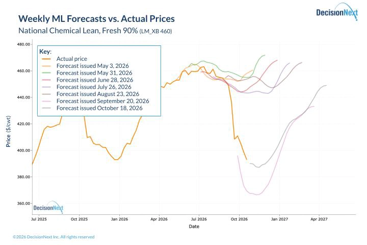
Figure 1 – Weekly machine-learning forecasts for domestic fresh 90% lean trim. Colored lines show forecasts generated on the dates listed; the ora

From July through August, the ML forecast consistently showed two things: a dip in values as we roll off the summer highs and a recovery toward high values toward the end of the year. This forecast model, which has had the best accuracy for this price series of the four weekly models over the last few years, did a good job capturing the relationship between 90% lean trim and other variables, as well as the series’ seasonality. However, at the longer horizon, the forecasts relied too heavily on the trend in beef prices established over the last five years. This overreliance is evident in the DecisionNext Tune Timeseries application, which shows the model’s variable selection focused heavily on the near term or could not find better long-term predictors than the strong upward trend (if you would like us to walk you through this in the software, reach out). 

This is a key reason why DecisionNext forecasts are not a black box; this information is valuable for investigating why forecasts are behaving the way they are. While we could use our expert opinion to suggest it was off and rebuild a new forecast model, the more we insert our expert opinion, the less new information the model is likely to show. We do not want our opinions to set our outlooks; we want our forecasts to define and challenge our assumptions. 

This is also why we value other forecast models to understand where prices are headed. We cannot simply force variables to select because it will make our forecasts worse and does not give us a consistent view of how the market changes. 

Here are the holdouts for the “Cutout” forecast for the 90% lean trim series (Fig. 2). The “Cutout” forecast technique is a three-part approach: first, forecast the cutout series; second, forecast the ratio of the trim value to the cutout; and lastly, combine the two through multiplication to get a “Cutout” forecast.

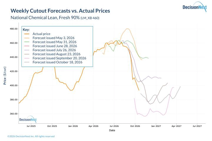
Figure 2 – Weekly Cutout-model forecasts for domestic fresh 90% lean trim. Colored lines show forecasts generated on the dates listed; the orange line shows actual prices.

This forecast was more aggressive than the ML forecast, suggesting a larger downturn in prices after the summer. This is because it better factored in the shift in beef demand, as well as expectations for lower cattle prices heading into the fall. 

Our last two models, “CME” and “Fundamentals,” use the same three-step approach as the Cutout model, substituting cattle prices for cutout prices. The approach for both models is: forecast cattle prices, forecast the trim-item-to-cattle-price ratio, then multiply them to estimate trim prices (Fig. 3). They differ only in how they forecast cattle prices: either the CME futures forward curves or a structural cattle model based on feeder cattle values, feed prices, and slaughter rates. The similar holdouts below strongly suggested a downward trend into fall.

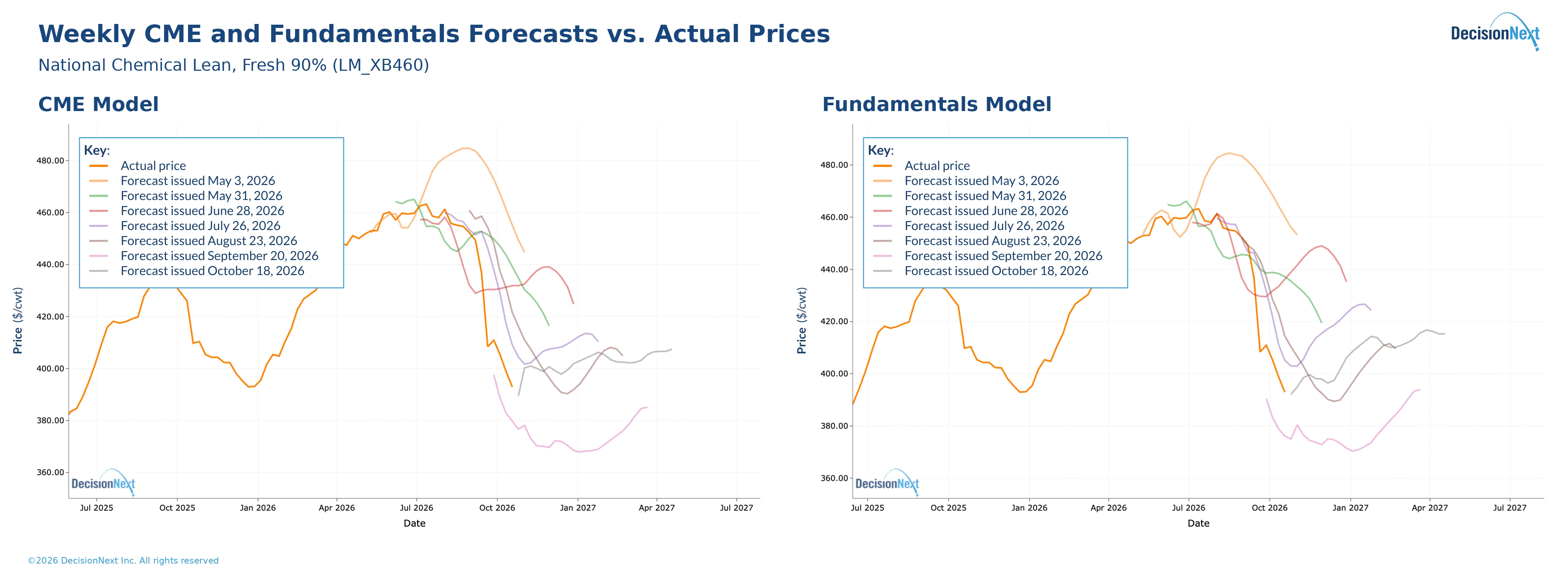
Figure 3 – Weekly CME-model (left) and Fundamentals-model (right) forecasts for domestic fresh 90% lean trim. Colored lines show forecasts generated on the dates listed; the orange line shows actual prices.

Although these forecasts largely align in the near term, we also track daily trim-market trends to be aware of rapid changes and confirm or reject the near-term pattern suggested above. Here are holdouts from the same machine-learning model applied to daily data (Fig. 4).

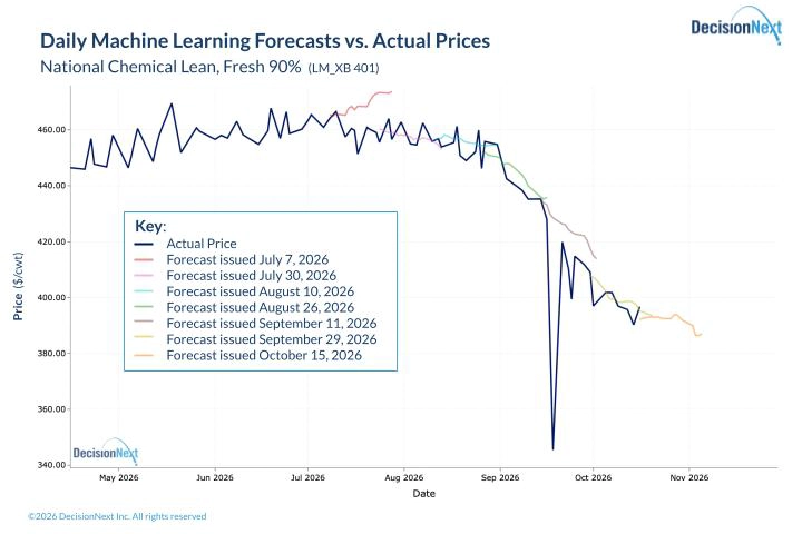
Figure 4 – Daily machine-learning forecasts for domestic fresh 90% lean trim. Colored lines show successive 15-business-day forecasts; the dark blue line shows actual prices.

The daily data is much noisier between observations, and we are only forecasting 15 business days out. Yet the trend in our forecasts continued to show downward price risk as we moved away from summer. This is consistent with the pattern seen in the more forward-looking weekly forecasts. 

Across these five forecasts, they generally agreed that prices would decline. The one thing they did not specify, though, was exactly when. While no model should reasonably be expected to do so all the time, market knowledge and additional data, such as indicators, can help confirm or refute the patterns. These indicators, though not always predictive, help us stay on top of relationships and changes in those relationships that might cause our outlook to shift. 

For 90% lean trim, the key indicators we track are:

• The relative value of steer versus cutter cow (Fig. 5A)

• The relative value of 90% trim versus cutter cows (Fig. 5B)

• The relative cost of domestic fresh versus imports (Fig. 5C)

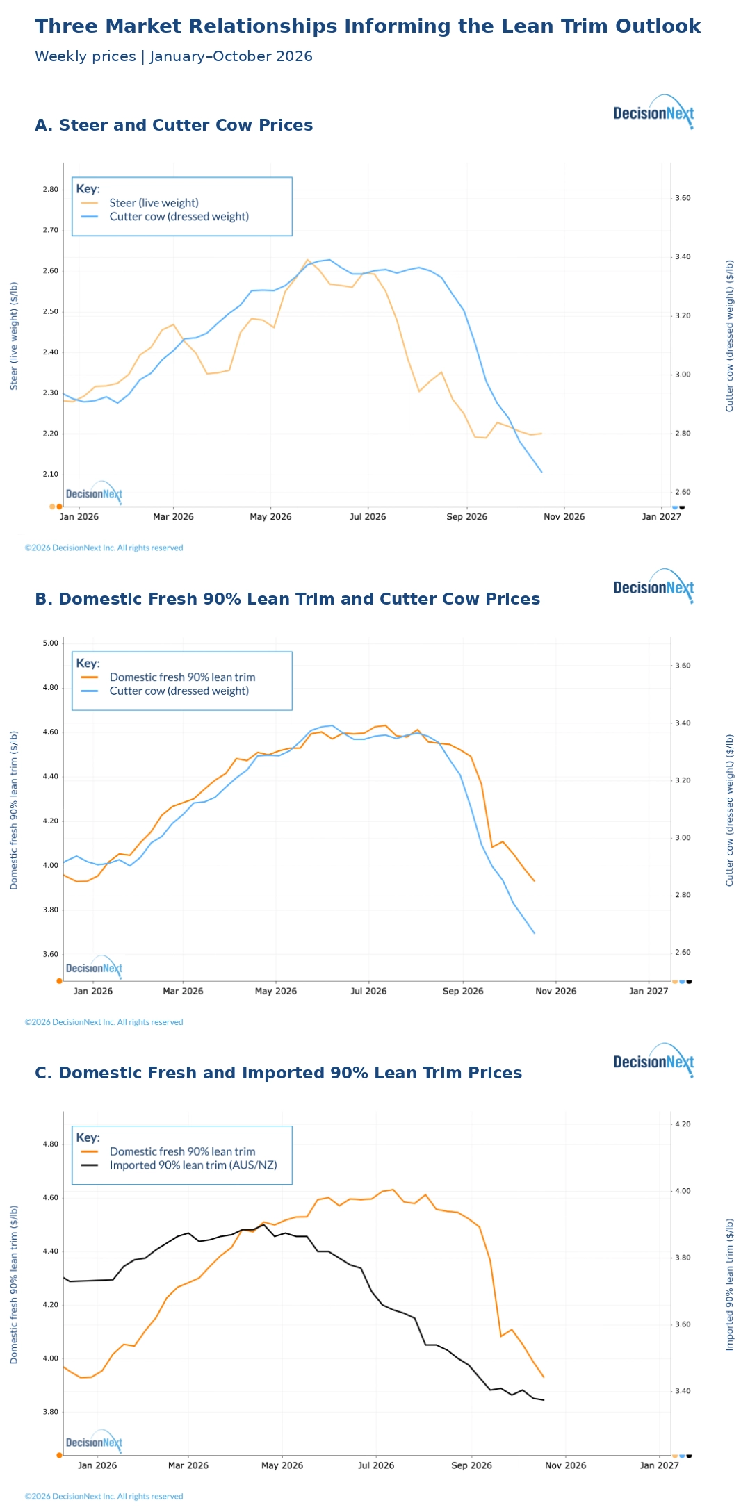
Figure 5 – Weekly price comparisons informing the domestic fresh 90% lean trim outlook: (A) steer and cutter cow prices, (B) domestic fresh trim and cutter cow prices, and (C) domestic fresh and imported trim prices. Each panel uses separate left and right price scales; compare the timing and direction of movements rather than the distance between lines.

We can see cattle prices falling, making cow values increasingly expensive (Fig. 5A). Although these two markets are clearly differentiated, they still track closely over time. Next, in the cow-and-trim comparison, cow prices fall quickly, followed by trim (Fig 5B). This is because some of trim’s seasonal pattern comes from cow supply. The cow moving ahead of trim highlights the supply component in the data series. Lastly, import trim values fall while domestic levels remain high (Fig. 5C). We know they are not perfect substitutes, and one moving while the other does not is not entirely indicative. Still, we can see the seasonal pattern in import trim, and the discount cannot keep widening forever—something has to give across all of these indicators.

Given that these five forecasts align on downward pressure, a fresh-beef buyer in July could have: (1) reduced forward purchases to preserve flexibility as prices decline, (2) shifted to import trim to capture the widening discount shown in the indicators, or (3) negotiated lower prices for forward commitments, using the forecast consensus as supporting evidence. Between the weeks ending July 26 and September 27, domestic fresh 90% lean trim prices declined by approximately $0.47/lb, or 10.3%, consistent with the downward pressure identified by the forecasts.

What if the models are not aligned?

While this decline in fresh 90% lean was clear from the data, in some instances forecasts or indicators don’t point in the same direction. But that is not a bad thing. It is telling us there are multiple factors driving the market, and we should evaluate those factors to know where it might go. While nuanced, this does not mean that one “forecast is wrong” but that something has to change for those forecasts to be realized. Remember from above, each model only sees a snippet of the market, and if we consider what they understand, then we can consider what is driving the market at any point in time. 

Suppose the ML and Cutout forecasts point higher while the CME and Fundamentals forecasts point lower. That pattern may suggest that cut-specific demand or carcass economics are providing more support than the cattle market implies.

If the cattle-linked forecasts are higher, tight cattle supplies or upstream market expectations may pose the larger upside risk. If ML is the outlier, the model may be capturing a cut-specific seasonal pattern, recent trend, or historical relationship not evident in the broader cattle and cutout outlooks. If CME is the outlier, futures-market expectations may diverge from signals in cash markets, carcass values, or the cut’s historical behavior. These interpretations are starting points, not automatic conclusions. 

Divergence is an invitation to investigate. 

The process can matter as much as the forecast

A forecast is not a crystal ball. No model will consistently get every market move right. Its value comes from helping us understand market conditions and supporting a rigorous decision-making process.

That process requires consistent study and evaluation of forecasts and related market indicators. When signals align, we have a stronger basis for acting. When the outlook is less clear, we can consider strategies that manage uncertainty and preserve flexibility. Rarely does a decision need to be all-or-nothing.

This is how we see around the market’s corners and plan business decisions around their outlook: by evaluating changing conditions consistently and adjusting our decisions as new information emerges.